Which representations do small models learn for finite-group multiplication?

Small models can be trained to multiply in a finite group and then generalise to element pairs they never saw during training. A few have been reverse-engineered to see what algorithm they found, and the readings disagree. On cyclic groups the model looks like it is doing a discrete Fourier transform (Nanda et al., 2023). On the symmetric groups $S_5$ and $S_6$ one team reads a representation-theoretic circuit¹1A representation sends each group element to an invertible matrix with $\rho(ab)=\rho(a)\rho(b)$, so composition becomes matrix multiplication. An irreducible one has no smaller subspace that every group element preserves; they are the pieces every other representation is built from. (Chughtai, Chan & Nanda, 2023) and another reads a coset route through the subgroup structure²2A coset $gH$ of a subgroup $H$ is one of the equal-sized, non-overlapping translates that tile the group. Asking which coset $ab$ falls in is a coarser question than asking what $ab$ is. (Stander et al., 2024).

On any single group these accounts are hard to tell apart, because several of them predict the same thing there. A reading on one group can say that some structured account fits, but not which one.

This project trains a controlled panel of groups of order 27 to 216 and asks, for each one, which part of the group’s structure the model uses. It also builds matched pairs of groups that the Fourier, tensor-rank, and coset accounts cannot tell apart, so that within a pair those accounts predict no difference and any difference the model does show counts against them.

Group multiplication is one of the few tasks whose correct algorithm is known exactly, which makes a model trained on it a testbed for interpretability tools themselves. A method that fails to recover structure we can write down has failed a check that models in the wild never offer.

What this study establishes

Small models trained to multiply in a finite group recruit only a small multiple of the minimal faithful amount³3A set of representations is faithful when only the identity acts trivially in all of them at once, so between them they still tell every pair of group elements apart. of the group’s representation-theoretic information, far below the whole regular representation⁴4The regular representation is the group acting on all functions from the group to $\mathbb{C}$, so it has dimension $|G|$. It contains every irreducible representation, each one repeated as many times as its dimension., which for any given group holds much more than the model needs. On the high-degree cells where the matrix-product test has power, the multi-layer-perceptron neurons do not build the product as a matrix multiplication over a shared index, and on the cells measured the read-position logits need no more than the scalar character of the irreducible representations the model uses. The blocks a model leans on carry causal weight, but on their own they do not reconstruct the model, so where the product is finally assembled is not something these measurements pin down.

On the matched pairs the competing accounts largely survive. Occupancy and recruited dimension show no within-pair difference, so on those readouts the accounts cannot be told apart. One readout, the sufficiency of the occupied blocks, shows a small within-pair difference on three pairs that survives correction for the number of comparisons made, a preliminary sign that the model uses structure the matched accounts hold fixed. I report it as a lead, not a settled falsification.

Any correct algorithm decomposes in the representation basis

Given a group $G$, a foundational result of representation theory states that the matrix entries of $G$‘s irreducible representations form a basis for functions from $G$ to $\mathbb{C}$, and products of those entries span functions of several group elements. Predicting the product is the same as evaluating the indicator $\mathbf{1}[ab=c]$, a function of the triple $(a,b,c)$, so any exact solution is some combination of that basis.

Because the basis is complete, though, every function on the group lies in its span, a lookup table included, so lying in the span says nothing about how a given model computes. Which irreducible representations a model concentrates on, and whether it uses their structure, is the empirical question the rest of the study measures.

The matched-pair instrument

The accounts of what these models compute are hard to separate because, on a single group, the Fourier decomposition, the tensor-rank structure, and the coset structure often point the same way. A matched pair breaks that tie. It is two groups identical on everything those accounts read. They share an ordinary character table⁵5The character table is the square array of character values, one row per irreducible representation and one column per conjugacy class. It pins down a great deal about a group, but not the group itself: non-isomorphic groups can share one., Frobenius-Schur indicators, and tensor-rank bounds, and no core-free subgroup⁶6A subgroup is core-free when it contains no non-trivial normal subgroup of the whole group. Its coset action sees the group in full, which is what makes such a subgroup usable by a coset algorithm., the kind of subgroup a coset action could exploit, tells them apart. The Fourier, tensor-rank, and coset accounts therefore all predict the two groups should behave identically on any measurement.

The two groups still differ in the structure those matched invariants leave free, their power-map structure, meaning which element is the square, cube, or higher power of which, and so each element’s order. A model that computed multiplication only from the structure the two groups share could not behave differently within a pair. Any reproducible within-pair difference is therefore structure the matched accounts cannot produce, and it counts against them.

This study measures six such pairs, the matched pairs that were trained. Separately, pairs that share a character table but differ in their Frobenius-Schur indicators, real against quaternionic⁷7The Frobenius-Schur indicator is $+1$, $0$ or $-1$ according to whether an irreducible representation is real, complex or quaternionic. The last two need more real dimension than their complex degree suggests, which is why $Q_8$ takes $4$ real dimensions for a degree-$2$ faithful representation., the Frobenius-Schur-flip pairs, serve as a positive control, since they are expected to differ, and a working instrument should find that difference where it exists.

Method

Every model here is a one-layer transformer trained on the group-multiplication task, at width 128 or 256. The training data is all $n^2$ ordered pairs of a group’s $n$ elements, each labelled with the index of its product read straight off the Cayley table⁸8The Cayley table is the full multiplication table of the group: an $n \times n$ grid whose $(a,b)$ entry is the product $ab$.. I train many random seeds of each group at each width, and call one such group-and-width combination a cell.

A seed enters the measurements only if it groks⁹9Grokking is when a model fits its training set early and only long afterwards switches to a solution that generalises, at which point held-out accuracy jumps., reaching essentially full accuracy on the non-leaked held-out pairs. Seeds that never grok are censored before any instrument runs, a little over a quarter of them across the panel, which is part of why cell counts vary.

A held-out pair can be leaked through its transpose when its two elements commute, so I measure generalisation only on the held-out pairs that are not transpose-leaked, and report the transpose-leak fraction as a covariate.

Every quantity is an estimate with a confidence interval from bootstrapping over seeds. There are no significance thresholds. A tight interval near zero is evidence against a large effect, and a wide interval means the measurement did not resolve anything.

Results

Not every instrument covers every group, so each result gives its own cell count.

How the model spreads its weight across irreducible representations

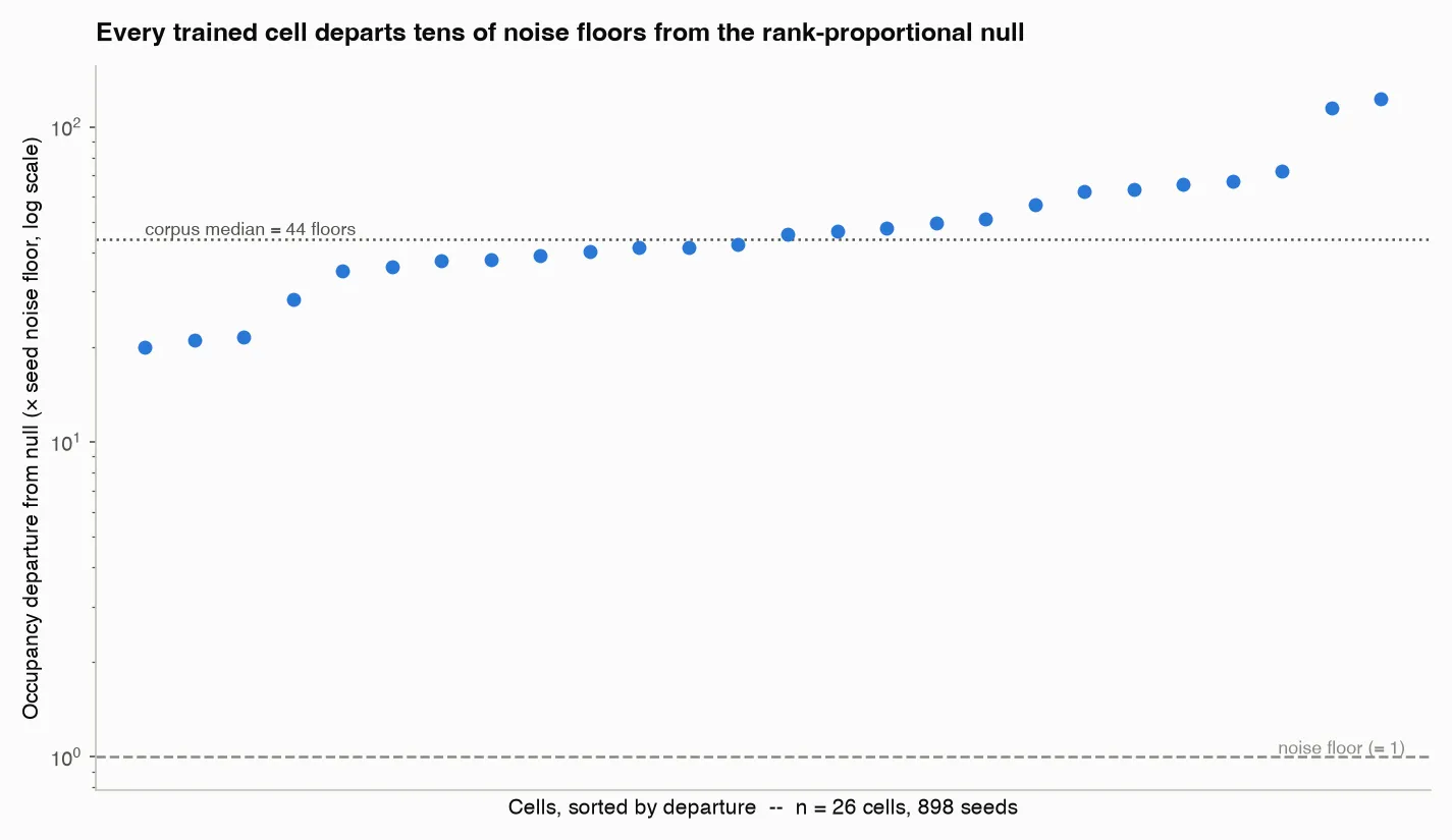
A structureless function of the inputs, with no group structure to exploit, would spread its activation energy across the isotypic blocks of the regular representation¹⁰10Grouping together all copies of one irreducible representation inside the regular representation gives its isotypic block. The blocks split the whole space into pieces no group element mixes. in proportion to each block’s rank. Instead every trained model piles its energy onto a few blocks.

Measured against the rank-proportional null, that spread sits a median total-variation distance of 0.558¹¹11Total-variation distance is the largest disagreement two distributions can show on any single event; $0$ means identical and $1$ means disjoint. away [0.517, 0.609] across the 26 cells, about 44 times the seed noise floor, which is a conservative planning scale, and no model comes close to the null. That rules out a structureless energy profile. A sparse, uneven spread is what almost any structured account predicts, the near-minimal-faithful thesis among them, so this shows the measurement catches structure without yet telling the accounts apart.

The effective dimension the model recruits

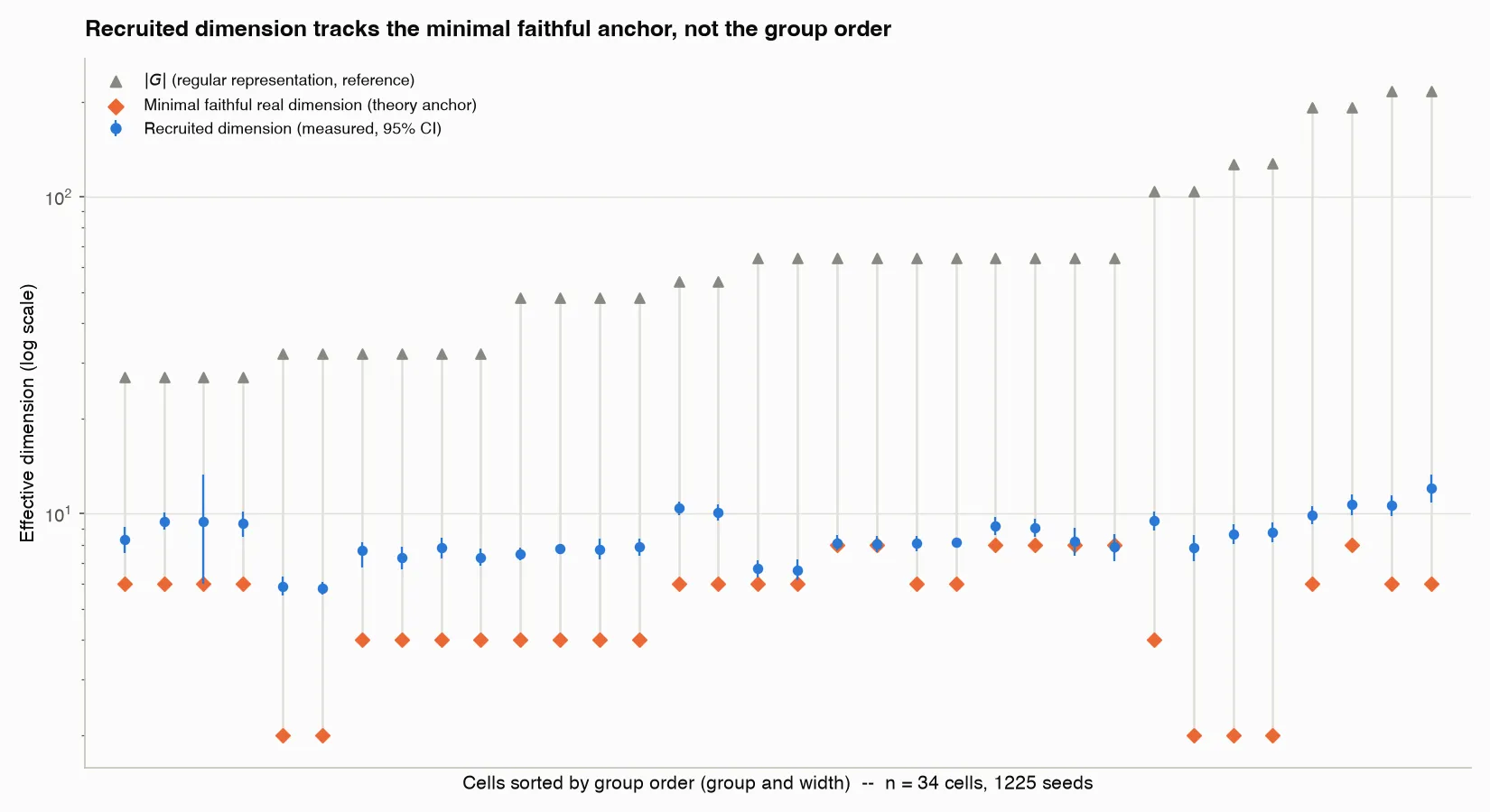
The effective dimension counts how many directions a model actually spreads over, through a participation ratio that rewards evenly shared variance, so a representation packed into a few directions scores low even when its raw rank is high. The low anchor is the minimal faithful real dimension, the smallest total real dimension of a set of irreducible representations whose direct sum is faithful, meaning their kernels meet only in the identity. The high anchor is the full regular representation, whose dimension is the group order.

Every model lands near the low anchor. Across 34 cells the effective dimension is 1.71 times the minimal faithful real dimension [1.39, 1.91] and about 14% of the group order (0.142 [0.125, 0.182]), and cell by cell it sits closer to the minimal-faithful anchor than to the group order in 1216 of 1225 seeds.

A model therefore recruits a small multiple of the minimal faithful dimension and a small fraction of the whole.

Whether the occupied blocks are the ones the model uses

Occupancy shows which blocks carry weight. Whether they do causal work is a separate matter. To test it, I ablate each isotypic block in turn and compare the drop in held-out accuracy against ablating a random subspace matched to that block in rank and norm.

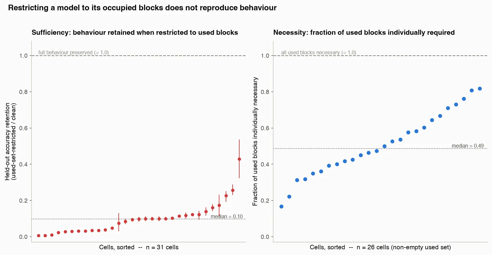
Ablating the block a model occupies most changes its held-out prediction on a median 0.185 more of the test pairs than the matched random subspace does [0.155, 0.208], positive in all 15 cells and concentrated in a few blocks. The blocks a model occupies are doing causal work beyond what a same-sized random subspace would.

Restricting a model to just its occupied blocks, everything outside them ablated, does not reproduce it. The restricted model keeps only a median 0.097 of its clean accuracy [0.037, 0.104], agrees with the intact model on about a tenth of held-out pairs, and its output distribution sits about 9 nats of Kullback-Leibler divergence away¹²12KL divergence measures how far one probability distribution sits from another, in nats when natural logarithms are used. Around $9$ nats is a very large gap for a distribution over a few hundred elements..

About half the used blocks are individually necessary beyond the random control, a median 0.487 [0.413, 0.590], and only 5 of 1082 seeds gave a set that was both sufficient and minimal.

The occupied blocks are load-bearing and mostly necessary, but on their own they do not rebuild the model, so the causal structure runs wider than occupancy alone marks out.

The matched-pair test

Applied within a matched pair, these panel instruments become a direct test of the competing accounts, since any reproducible within-pair difference is something those accounts cannot explain.

On occupancy the pairs are indistinguishable, every measured pair’s within-pair difference in energy spread spanning zero, and recruited dimension spans zero on every matched pair too. The Frobenius-Schur-flip pairs show the recruited-dimension instrument can find a difference when one is there, its within-pair difference on those pairs large and clear of zero, for example -1.53 [-1.95, -1.14]. That control establishes sensitivity for the recruited-dimension readout. Occupancy and the used-set readout below have no matched control of their own, so their within-pair nulls are read without that check.

One readout breaks the pattern. On three of the matched pairs, (27,3)/(27,4), (64,74)/(64,80) and (64,228)/(64,229)¹³13Groups are named by GAP SmallGroup id: $(n,k)$ is the $k$-th group of order $n$ in the standard catalogue of all groups of that order., restricting a model to the isotypic blocks it occupies leaves a different amount of its accuracy standing in one group than in the other. The margin is small, around two to three points of retained accuracy, comparable to the ordinary seed-to-seed spread within a single cell, but it survives a Benjamini-Hochberg correction¹⁴14The Benjamini-Hochberg procedure adjusts a whole battery of tests together, so that the expected share of false positives among the results called significant stays bounded. across the whole battery of within-pair contrasts. Occupancy and recruited dimension can match within a pair while this differs because they measure different things, how much weight each block carries against whether those blocks are jointly enough to rebuild the model. The necessity side of the same audit does not corroborate the difference. I read it as a preliminary lead, structure the model uses that the matched accounts hold fixed, worth an attribution follow-up before it could be called a falsification.

Whether the neurons form the matrix product

The representation account says a model embeds each element as its irreducible-representation matrices, multiplies the matrix for $a$ by the matrix for $b$ to get the matrix for the product, and reads the answer off through a character¹⁵15A character is $\chi(g)=\operatorname{tr}\rho(g)$, the trace of the representation matrix. It is constant on each conjugacy class, so it is a coarser record than the matrix it came from.. The step that can be tested is the middle one, a matrix product formed in the neurons. To look for it, I take the grid of hidden pre-activations, one vector per ordered pair of inputs, and fit three nested forms to it out of sample.

The first is the shared-index matrix product the account predicts, where the matrix for $a$ and the matrix for $b$ are multiplied over one shared index¹⁶16In a matrix product every term is $\sum_j \rho(a)_{ij}\rho(b)_{jk}$: the second index of the first matrix is tied to the first index of the second. Drop that constraint and the two matrices’ entries may meet in any pairing at all.. The second is a generic bilinear form, which lets the two arguments’ matrix entries interact through any pair of indices and so drops the shared-index constraint. The third is a saturated ceiling, free to be any function of the product $ab$. I fit the coefficients freely, so no choice of basis for the representation affects the reading.

Across the four cells where the relevant irreducible representation has degree three or four, (192,10), (192,24), (216,106) and (216,107) at width 128, the matrix-product form is credited on no block of any cell, over 48 to 50 seeds each. A saturated form free to be any function of the product explains up to about 0.12 of held-out variance, so only a small share of the neurons’ pre-activation variance tracks the product at all. Against that ceiling the constrained matrix product and the generic bilinear form explain almost none of it, at most about 0.01 and 0.02.

On these four high-degree cells the neurons’ pre-activations hold no linearly recoverable shared-index matrix product, and the generic bilinear form recovers no more. The low ceiling means the product itself is only weakly present in them.

What the readout reads

The neurons do not carry the product as a shared-index matrix product, so the next question is what the output stage needs in order to name it.

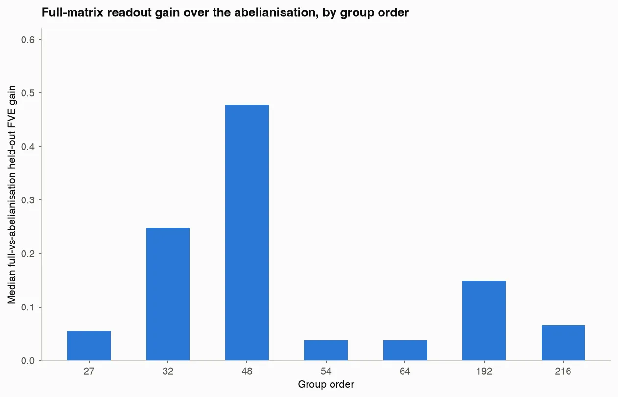
One comparison sets the full irreducible-representation matrices against a readout that keeps only the one-dimensional characters, the abelianisation¹⁷17One-dimensional characters send each element to a single number. They factor through the abelianisation $G/[G,G]$, the largest commutative quotient of the group, obtained by declaring $ab$ and $ba$ equal, so they see its commutative shadow and nothing finer.. At orders 64 and below the median gain from the full matrices is 0.067 of held-out variance explained [0.043, 0.180], and it depends on the group, small at orders 27, 54 and 64 but larger at the smaller orders 32 and 48, around 0.25 and 0.48, with no simple relationship to order.

At orders 192 and 216, over 48 to 50 seeds, the gain stays positive, 0.177 [0.154, 0.20] and 0.122 [0.107, 0.14] at order 192 and 0.066 at both order-216 cells ([0.057, 0.075] and [0.058, 0.075]). The higher-dimensional irreducible representations carry something the abelianisation throws away.

A second sets the full matrix entries against just the scalar character of the same irreducible representations. Now the extra gain is small, 0.037 [0.029, 0.045] at (216,106), 0.035 [0.027, 0.044] at (216,107) and 0.046 [0.038, 0.055] at (64,60), over 48 to 50 seeds. The scalar character carries most of what the readout uses, and the full matrix entries add only a little more. Because the character of a product is a function of that product, this fit is consistent with any algorithm that computes the group operation correctly, so it shows the readout needs no more than the character and does not localise where the product is assembled.

The coset route as a concrete instance

A model can carry a small coordinate that tracks which coset of a normal subgroup¹⁸18A subgroup $N$ is normal when $gNg^{-1}=N$ for every $g$, which is what lets its cosets be multiplied as a group in their own right. an element sits in, and use it to work out which coset the product lands in. The functions constant on the cosets of a normal subgroup span a low-rank subspace, one coordinate per element of the quotient¹⁹19Collapsing a normal subgroup $N$ to a point leaves the quotient group $G/N$, whose elements are the cosets of $N$. It is a smaller group that remembers only part of $G$., a small piece of representation-theoretic structure with a specific job.

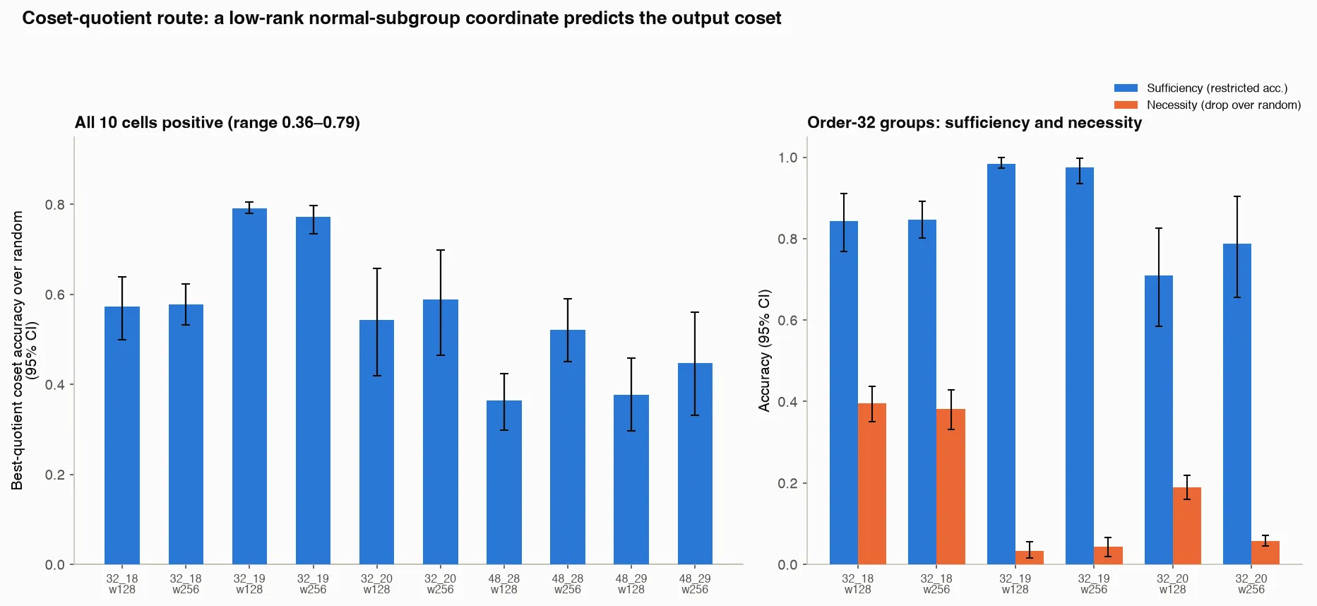
For each group the instrument finds the normal-subgroup quotient whose coordinate best predicts the product’s coset, and tests it against a matched random subspace of the same rank. Sufficiency restricts each element’s embedding to its coset average and asks whether the model still gets the product’s coset right. Necessity ablates the coordinate and measures how far coset accuracy falls. Across all ten measured cells, at orders 32 and 48, that coordinate beats its control by 0.36 to 0.79, every interval clear of zero. Across the order-32 groups it is largely sufficient on its own, holding coset prediction at 0.71 to 0.98, and removing it costs 0.03 to 0.40.

A model therefore does work with a small quotient coordinate, exactly the kind of near-minimal faithful piece the rest of the study describes. A coset coordinate is itself built from the group’s character blocks, so it cannot on its own pull the coset reading apart from the representation reading.

Limitations

The scope is narrow. Every model here is a one-layer transformer at one of two widths, trained on finite groups of order 27 to 216. Cross-group comparisons are associations between separately trained models, so none of them pins a difference to a single cause. The set of groups is small, so any statement is about these particular groups, and a population-level claim stays out of reach.

Near-minimal is a loose description. The dimension a model recruits sits at about 1.7 times the minimal faithful real dimension across the panel. That is far below the full regular representation and close to the minimal faithful set, without sitting exactly on it.

The readout is not fully pinned down. The scalar character carries most of what the output stage reads, but the full matrix entries add a small, reliably positive amount on top, a full-over-character gain of 0.035 to 0.046 on the cells measured. The full-over-abelianisation comparison is also partial, with the group-by-group breakdown resolved only at orders 64 and below.

The two negative results, that the neurons hold no shared-index matrix product and that the readout needs no more than the character, come from the handful of cells where each test has power, four cells and three, a small subset of the panel.

The matched-pair test rests on six pairs, and the one within-pair difference it turns up, on used-set sufficiency, is a preliminary signal. It is small, about one seed’s worth of scatter, the necessity side of the same audit does not back it up, and it is one clearing result among many comparisons. Confirming or dismissing it wants more seeds and a measurement aimed at the power-map structure the pairs vary, which would say whether the difference is really that structure at work.

What the testbed is for

The matched-pair instrument shows what this testbed buys. Its Frobenius-Schur-flip control catches the difference it is built to catch, the calibration any method deserves before it is used on a model whose ground truth no one can write down. The specific findings are about small transformers on finite groups, but measuring against a known answer with a matched control is the part that carries over.

Reproducibility and method notes

All the instrument analysis runs against saved checkpoints from a finished training campaign. Every reading records which model and which checkpoint it came from, through a manifest system. Any number in this write-up traces back to the run that produced it and can be re-derived from the same artefact.

Appendix: the groups

Every group trained on and drawn on in the results above²⁰20In the Structure column $\times$ is a direct product, $:$ a semidirect product and $.$ a non-split extension; $C_n$ is cyclic of order $n$, $D_n$ dihedral of order $n$, $Q_n$ generalised quaternion and $QD_n$ quasidihedral., all of order 27 to 216. The last column is the largest dimension among a group’s irreducible representations, which sets whether the matrix-product test has anything above one dimension to look at.

Group	Structure	Largest irrep degree
(27,3)	(C3 x C3) : C3	3
(27,4)	C9 : C3	3
(32,18)	D32, dihedral of order 32	2
(32,19)	QD32, quasidihedral	2
(32,20)	Q32, generalised quaternion	2
(48,28)	SL(2,3) . C2	4
(48,29)	GL(2,3)	4
(54,10)	C2 x ((C3 x C3) : C3)	3
(54,11)	C2 x (C9 : C3)	3
(64,60)	(C2 x ((C4 x C2) : C2)) : C2	2
(64,65)	(C4 x C4) : C4	2
(64,74)	((C4 x C2) : C4) : C2	2
(64,80)	((C4 x C2) : C4) : C2	2
(64,228)	(C2 x ((C4 x C2) : C2)) : C2	4
(64,229)	(C2 x ((C4 x C2) : C2)) : C2	4
(64,236)	((C4 x C4) : C2) : C2	4
(64,240)	(C4 x D8) : C2	4
(64,241)	((C4 x C2 x C2) : C2) : C2	4
(64,242)	((C4 x C4) : C2) : C2	4
(104,4)	C13 : Q8	2
(104,6)	D104, dihedral of order 104	2
(127,1)	C127, cyclic	1
(128,1)	C128, cyclic	1
(128,2328)	(C2)^7, elementary abelian	1
(192,10)	C3 : (((C4 x C2) : C4) : C2)	4
(192,24)	C3 : ((C2 x C2) . ((C4 x C2) : C2))	4
(216,106)	C2 x ((C2 x C2) : (C9 : C3))	3
(216,107)	C2 x ((C2 x C2) : ((C3 x C3) : C3))	3

The matched pairs measured are (27,3)/(27,4), (54,10)/(54,11), (64,74)/(64,80), (64,228)/(64,229), (64,236)/(64,240) and (64,241)/(64,242). The Frobenius-Schur-flip control pairs, which share a character table but are expected to differ, are (32,18)/(32,20), (64,60)/(64,65) and (104,4)/(104,6).

Some matched pairs share a Structure string here, for example (64,74)/(64,80) and (64,228)/(64,229). That decomposition does not capture the power-map structure that tells the pair apart.

Comments

Comments are moderated; no account needed.

Name

Comment

Leave this field empty

Post comment